Parse
While {MIPTools} provides several .csv files that can be analyzed, parsing such files is difficult because of their non-rectangular structure. As such, attempting to read these files with default parameters fails.
#> # A tibble: 10 × 5
#>    X1            X2               X3               X4               X5
#>    <chr>         <chr>            <chr>            <chr>            <chr>
#>  1 Gene ID       PF3D7_0106300    PF3D7_0106300    PF3D7_0106300    PF3D7_01063…
#>  2 Gene          atp6             atp6             atp6             atp6
#>  3 Mutation Name atp6-Ala623Glu   atp6-Glu431Lys   atp6-Gly639Asp   atp6-Ser466…
#>  4 ExonicFunc    missense_variant missense_variant missense_variant missense_va…
#>  5 AA Change     Ala623Glu        Glu431Lys        Gly639Asp        Ser466Asn
#>  6 Targeted      Yes              Yes              No               No
#>  7 D10-JJJ-23    608.0            699.0            608.0            237.0
#>  8 D10-JJJ-43    20.0             30.0             20.0             0.0
#>  9 D10-JJJ-55    158.0            242.0            158.0            61.0
#> 10 D10-JJJ-5     2.0              9.0              2.0              1.0
As visible, there are six rows of metadata, which specify the gene ID, gene, mutation name, etc. The remaining rows contain the data we are actually interested in: the rows contain the samples and the columns contain the positions we are interested in. The difficult part of reading in these files is that the metadata must be extracted and treated differently from the data itself.
miplicorn, therefore, provides a family of functions: read_tbl_*() which quickly read in such non-rectangular files. The functions generate a tibble where each row represents a sample and a position. Thus, there will be multiple entries for each unique sample.
cov_file <- miplicorn::miplicorn_example("coverage_AA_table.csv")

data <- miplicorn::read_tbl_coverage(cov_file)
data
#> # A tibble: 6,344 × 8
#>    sample    gene_id gene  mutation_name exonic_func aa_change targeted coverage
#>    <chr>     <chr>   <chr> <chr>         <chr>       <chr>     <chr>       <dbl>
#>  1 D10-JJJ-… PF3D7_… atp6  atp6-Ala623G… missense_v… Ala623Glu Yes           608
#>  2 D10-JJJ-… PF3D7_… atp6  atp6-Ala623G… missense_v… Ala623Glu Yes            20
#>  3 D10-JJJ-… PF3D7_… atp6  atp6-Ala623G… missense_v… Ala623Glu Yes           158
#>  4 D10-JJJ-5 PF3D7_… atp6  atp6-Ala623G… missense_v… Ala623Glu Yes             2
#>  5 D10-JJJ-… PF3D7_… atp6  atp6-Ala623G… missense_v… Ala623Glu Yes             1
#>  6 D10-JJJ-… PF3D7_… atp6  atp6-Ala623G… missense_v… Ala623Glu Yes           129
#>  7 D10-JJJ-… PF3D7_… atp6  atp6-Ala623G… missense_v… Ala623Glu Yes             0
#>  8 D10-JJJ-… PF3D7_… atp6  atp6-Ala623G… missense_v… Ala623Glu Yes             0
#>  9 D10-JJJ-… PF3D7_… atp6  atp6-Ala623G… missense_v… Ala623Glu Yes            90
#> 10 D10-JJJ-… PF3D7_… atp6  atp6-Ala623G… missense_v… Ala623Glu Yes           175
#> # … with 6,334 more rows
Manipulate
Amino acids
In some the user may want to convert amino acid abbreviations from the three to one letters abbreviation, or vice versa for easier interpretation of data.
data %>%
  dplyr::mutate(aa_change = convert_three(aa_change))
#> # A tibble: 6,344 × 8
#>    sample    gene_id gene  mutation_name exonic_func aa_change targeted coverage
#>    <chr>     <chr>   <chr> <chr>         <chr>       <chr>     <chr>       <dbl>
#>  1 D10-JJJ-… PF3D7_… atp6  atp6-Ala623G… missense_v… A623E     Yes           608
#>  2 D10-JJJ-… PF3D7_… atp6  atp6-Ala623G… missense_v… A623E     Yes            20
#>  3 D10-JJJ-… PF3D7_… atp6  atp6-Ala623G… missense_v… A623E     Yes           158
#>  4 D10-JJJ-5 PF3D7_… atp6  atp6-Ala623G… missense_v… A623E     Yes             2
#>  5 D10-JJJ-… PF3D7_… atp6  atp6-Ala623G… missense_v… A623E     Yes             1
#>  6 D10-JJJ-… PF3D7_… atp6  atp6-Ala623G… missense_v… A623E     Yes           129
#>  7 D10-JJJ-… PF3D7_… atp6  atp6-Ala623G… missense_v… A623E     Yes             0
#>  8 D10-JJJ-… PF3D7_… atp6  atp6-Ala623G… missense_v… A623E     Yes             0
#>  9 D10-JJJ-… PF3D7_… atp6  atp6-Ala623G… missense_v… A623E     Yes            90
#> 10 D10-JJJ-… PF3D7_… atp6  atp6-Ala623G… missense_v… A623E     Yes           175
#> # … with 6,334 more rows
Sort
In plotting data, it is useful to be able to control the order in which data appears. While dplyr::arrange() provides the functionality to sort numeric or character data, it lacks the ability to naturally sort alphanumeric vectors, vectors containing both letters and numerics. Furthermore, the ordering of data is not kept when fed into plotting functions. arrange_natural() attempts to address these limitations.
arrange_natural(data, sample, gene)
#> # A tibble: 6,344 × 8
#>    sample    gene_id gene  mutation_name exonic_func aa_change targeted coverage
#>    <fct>     <chr>   <fct> <chr>         <chr>       <chr>     <chr>       <dbl>
#>  1 D10-JJJ-1 PF3D7_… atp6  atp6-Ala623G… missense_v… Ala623Glu Yes            10
#>  2 D10-JJJ-1 PF3D7_… atp6  atp6-Glu431L… missense_v… Glu431Lys Yes             5
#>  3 D10-JJJ-1 PF3D7_… atp6  atp6-Gly639A… missense_v… Gly639Asp No             10
#>  4 D10-JJJ-1 PF3D7_… atp6  atp6-Ser466A… missense_v… Ser466Asn No              2
#>  5 D10-JJJ-1 PF3D7_… atp6  atp6-Ser769A… missense_v… Ser769Asn Yes             1
#>  6 D10-JJJ-1 PF3D7_… crt   crt-Ala220Ser missense_v… Ala220Ser Yes             2
#>  7 D10-JJJ-1 PF3D7_… crt   crt-Asn326Asp missense_v… Asn326Asp No              2
#>  8 D10-JJJ-1 PF3D7_… crt   crt-Asn326Ser missense_v… Asn326Ser Yes             2
#>  9 D10-JJJ-1 PF3D7_… crt   crt-Asn75Glu  missense_v… Asn75Glu  Yes             0
#> 10 D10-JJJ-1 PF3D7_… crt   crt-Cys72Ser  missense_v… Cys72Ser  Yes             0
#> # … with 6,334 more rows
Visualize
There are an almost limitless different ways to visualize a single set of data. While miplicorn cannot address every method, it aims to simplify the creation of key figures.
Chromosome map
There are two built in ways to create chromosome maps, each with its own set of strengths and weaknesses. You can either make an interactive map or a more detailed karyoplot.
colours <- c("#006A8EFF", "#A8A6A7FF", "#B1283AFF")
map <- plot_chromoMap(genome_Pf3D7, probes, colours = colours)

# Used to embed into html
widgetframe::frameableWidget(map)
plot_karyoploteR(genome_Pf3D7, probes, colours = colours)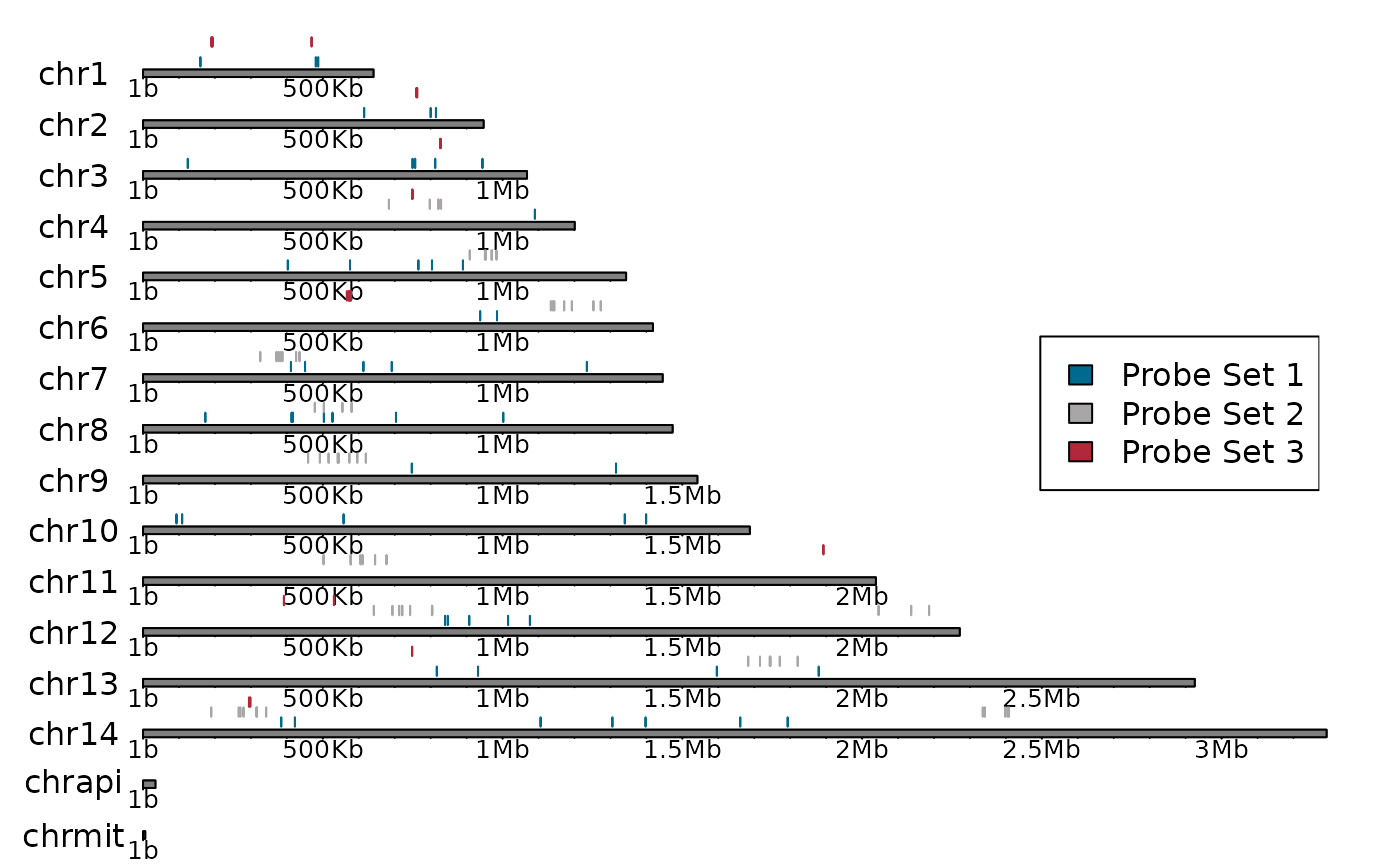
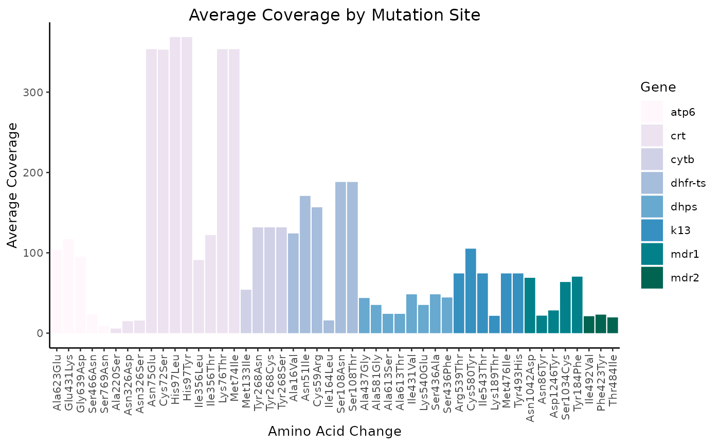
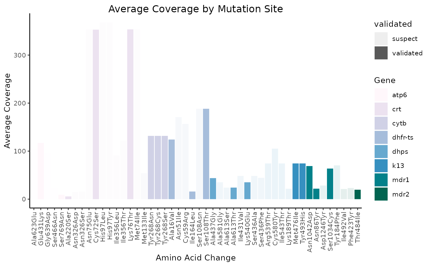
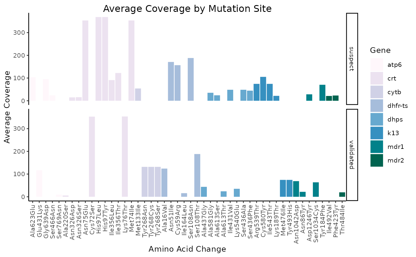
Average coverage
N.B. the remaining figures have not yet been incorporated into miplicorn, but as time goes on, more and more visualization methods will be added.