Continuous sensitivity analysis
Source:vignettes/sensitivity_analysis_continuous.Rmd
sensitivity_analysis_continuous.RmdIntroduction
In this analysis file, we aim to understand the effect of varying parameters on our COI framework. We will examine both simulation and estimation parameters. The parameters that we will examine are:
-
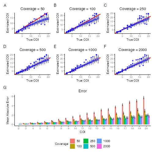
coverage: Coverage at each locus. -
loci: The number of loci. -
alpha: Shape parameter of the symmetric Dirichlet prior on strain proportions. -
overdispersion: The extent to which counts are over-dispersed relative to the binomial distribution. Counts are Beta-binomially distributed, with the beta distribution having shape parameters \(p/\text{overdispersion}\) and \((1-p) / \text{overdispersion}\). -
relatedness: The probability that a strain in mixed infections is related to another. -
epsilon: The probability of a single read being miscalled as the other allele. Applies in both directions. -
coi: The complexity of infection of the sample. -
seq_error: The level of sequencing error that is assumed. -
use_bins: Whether or not to group data before estimating the COI. -
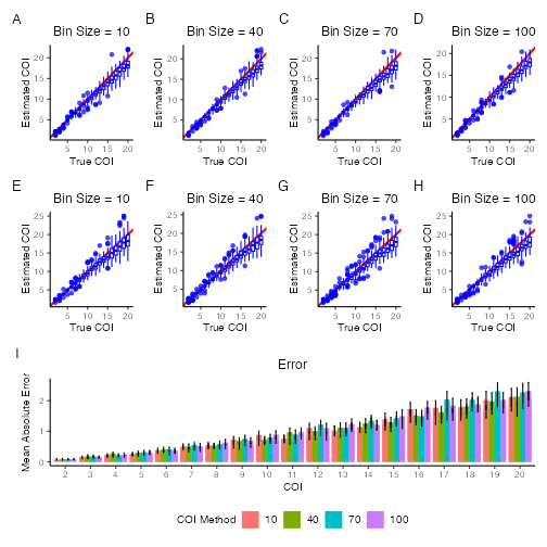
bin_size: The minimum size of each bin of data.
Default parameters
| Parameter | Default Value |
|---|---|
| COI | 3 |
| PLMAF | runif(1000, 0, 0.5) |
| Coverage | 200 |
| Alpha | 1 |
| Overdispersion | 0 |
| Relatedness | 0 |
| Epsilon | 0 |
| Sequence Error | 0.01 |
| Use Bins | FALSE |
| Bin Size | 20 |
Overall performance
toverall <- cont_sensitivity(
  coi = 1:20,
  repetitions = 100,
  plmaf = p,
  coverage = 200,
  seq_error = 0,
  coi_method = c("variant", "frequency")
)

toverall_image <- sensitivity_plot(
  data = toverall,
  dims = c(1, 2),
  result_type = "cont",
  title = "Predicted COI",
  sub_title = c("Variant Method", "Frequency Method")
)

toverall_error <- error_plot(
  data = toverall,
  fill = "coi_method",
  legend_title = "COI Method",
  title = "Error",
  fill_levels = c("Variant Method", "Frequency Method")
)

toverall_fig <- toverall_image / toverall_error +
  plot_annotation(
    tag_levels = "A",
    theme = theme(plot.tag = element_text(size = 10))
  ) +
  theme(legend.position = "bottom")

toverall_fig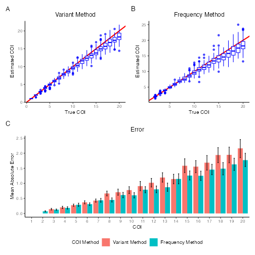
Simulation parameters
Coverage
tcoverage_1 <- cont_sensitivity(
  coi = 2:20,
  coverage = c(50, 100, 250, 500, 1000, 2000),
  repetitions = 100,
  seq_error = 0.01,
  plmaf = p,
  coi_method = "variant"
)

tcoverage_image_1 <- sensitivity_plot(
  data = tcoverage_1,
  result_type = "cont",
  title = "Predicted COI",
  dims = c(2, 3),
  sub_title = paste0("Coverage = ", c(50, 100, 250, 500, 1000, 2000))
)

tcoverage_error_1 <- error_plot(
  tcoverage_1,
  fill = "coverage",
  legend_title = "Coverage",
  title = "Error"
)

tcoverage_fig_1 <- tcoverage_image_1 / tcoverage_error_1 +
  plot_annotation(
    tag_levels = "A",
    theme = theme(plot.tag = element_text(size = 10))
  ) +
  plot_layout(heights = c(2, 1)) +
  theme(legend.position = "bottom")

tcoverage_fig_1
tcoverage_2 <- cont_sensitivity(
  coi = 2:20,
  coverage = c(50, 100, 250, 500, 1000, 2000),
  repetitions = 100,
  seq_error = 0.01,
  plmaf = p,
  coi_method = "frequency"
)

tcoverage_image_2 <- sensitivity_plot(
  data = tcoverage_2,
  result_type = "cont",
  title = "Predicted COI",
  dims = c(2, 3),
  sub_title = paste0("Coverage = ", c(50, 100, 250, 500, 1000, 2000))
)

tcoverage_error_2 <- error_plot(
  tcoverage_2,
  fill = "coverage",
  legend_title = "Coverage",
  title = "Error"
)

tcoverage_fig_2 <- tcoverage_image_2 / tcoverage_error_2 +
  plot_annotation(
    tag_levels = "A",
    theme = theme(plot.tag = element_text(size = 10))
  ) +
  plot_layout(heights = c(2, 1)) +
  theme(legend.position = "bottom")

tcoverage_fig_2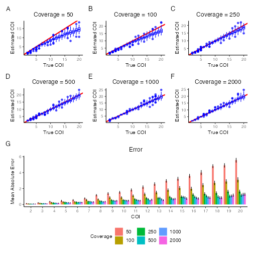
Loci
# Set the range over which we will iterate
loci <- c(1e2, 1e3, 1e4)

# For each loci, reset the PLMAF and then run
bloci <- lapply(loci, function(new_L) {
  new_p <- rbeta(new_L, 1, 5)
  new_p[new_p > 0.5] <- 1 - new_p[new_p > 0.5]

  inner_tloci <- cont_sensitivity(
    coi = 2:20,
    repetitions = 100,
    plmaf = new_p,
    seq_error = 0.01,
    coi_method = "variant"
  )
  inner_tloci$param_grid$loci <- new_L
  return(inner_tloci)
})

# Extract the relevant information for each output: predicted_coi, probability,
# param_grid, and boot_error
pc <- do.call(cbind, lapply(bloci, function(test) {
  return(test$predicted_coi)
}))
pb <- do.call(cbind, lapply(bloci, function(test) {
  return(test$probability)
}))
pg <- do.call(rbind, lapply(bloci, function(test) {
  return(test$param_grid)
}))
be <- do.call(rbind, lapply(bloci, function(test) {
  return(test$boot_error)
}))

# Fix the naming for predicted_coi
num_cois <- length(unique(pg$coi))
num_repeat_cois <- length(pg$coi) / num_cois
names(pc) <- paste(
  "coi",
  pg$coi,
  rep(seq(num_repeat_cois), each = num_cois),
  sep = "_"
)

# Create the output
tloci_1 <- list(
  predicted_coi = pc,
  probability   = pb,
  param_grid    = pg,
  boot_error    = be
)

# Plot
tloci_image_1 <- sensitivity_plot(
  data = tloci_1,
  result_type = "cont",
  title = "Predicted COI",
  dims = c(1, 3),
  sub_title = paste0("Loci = ", c(1e2, 1e3, 1e4))
)

# Add a loci column
tloci_1$boot_error$loci <- rep(
  c(1e2, 1e3, 1e4),
  each = length(unique(tloci_1$boot_error$coi))
)
tloci_error_1 <- error_plot(
  tloci_1,
  fill = "loci",
  legend_title = "Loci",
  title = "Error"
)

tloci_fig_1 <- tloci_image_1 / tloci_error_1 +
  plot_annotation(
    tag_levels = "A",
    theme = theme(plot.tag = element_text(size = 10))
  ) +
  theme(legend.position = "bottom")

tloci_fig_1
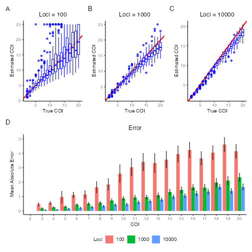
# Set the range over which we will iterate
loci <- c(1e2, 1e3, 1e4)

# For each loci, reset the PLMAF and then run
bloci <- lapply(loci, function(new_L) {
  new_p <- rbeta(new_L, 1, 5)
  new_p[new_p > 0.5] <- 1 - new_p[new_p > 0.5]

  inner_tloci <- cont_sensitivity(
    coi = 2:20,
    repetitions = 100,
    plmaf = new_p,
    seq_error = 0.01,
    coi_method = "frequency"
  )
  inner_tloci$param_grid$loci <- new_L
  return(inner_tloci)
})

# Extract the relevant information for each output: predicted_coi, probability,
# param_grid, and boot_error
pc <- do.call(cbind, lapply(bloci, function(test) {
  return(test$predicted_coi)
}))
pb <- do.call(cbind, lapply(bloci, function(test) {
  return(test$probability)
}))
pg <- do.call(rbind, lapply(bloci, function(test) {
  return(test$param_grid)
}))
be <- do.call(rbind, lapply(bloci, function(test) {
  return(test$boot_error)
}))

# Fix the naming for predicted_coi
num_cois <- length(unique(pg$coi))
num_repeat_cois <- length(pg$coi) / num_cois
names(pc) <- paste(
  "coi",
  pg$coi,
  rep(seq(num_repeat_cois), each = num_cois),
  sep = "_"
)

# Create the output
tloci_2 <- list(
  predicted_coi = pc,
  probability   = pb,
  param_grid    = pg,
  boot_error    = be
)

# Plot
tloci_image_2 <- sensitivity_plot(
  data = tloci_2,
  result_type = "cont",
  title = "Predicted COI",
  dims = c(1, 3),
  sub_title = paste0("Loci = ", c(1e2, 1e3, 1e4))
)

# Add a loci column
tloci_2$boot_error$loci <- rep(
  c(1e2, 1e3, 1e4),
  each = length(unique(tloci_2$boot_error$coi))
)
tloci_error_2 <- error_plot(
  tloci_2,
  fill = "loci",
  legend_title = "Loci",
  title = "Error"
)

tloci_fig_2 <- tloci_image_2 / tloci_error_2 +
  plot_annotation(
    tag_levels = "A",
    theme = theme(plot.tag = element_text(size = 10))
  ) +
  theme(legend.position = "bottom")

tloci_fig_2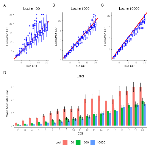
Alpha
talpha_1 <- cont_sensitivity(
  coi = 2:20,
  alpha = seq(0.01, 5.51, 0.5),
  repetitions = 100,
  seq_error = 0.01,
  plmaf = p
)

talpha_image_1 <- sensitivity_plot(
  data = talpha_1,
  result_type = "cont",
  title = "Predicted COI",
  dims = c(4, 3),
  sub_title = paste0("Alpha = ", seq(0.01, 5.51, 0.5))
)

talpha_error_1 <- error_plot(
  talpha_1,
  fill = "alpha",
  legend_title = "Alpha",
  title = "Error"
)

talpha_fig_1 <- talpha_image_1 / talpha_error_1 +
  plot_annotation(
    tag_levels = "A",
    theme = theme(plot.tag = element_text(size = 10))
  ) +
  plot_layout(heights = c(5, 1)) +
  theme(legend.position = "bottom")

talpha_fig_1
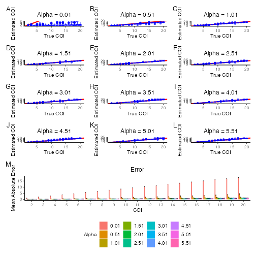
talpha_2 <- cont_sensitivity(
  coi = 2:20,
  alpha = seq(0.01, 5.51, 0.5),
  repetitions = 100,
  seq_error = 0.01,
  plmaf = p
)

talpha_image_2 <- sensitivity_plot(
  data = talpha_2,
  result_type = "cont",
  title = "Predicted COI",
  dims = c(4, 3),
  sub_title = paste0("Alpha = ", seq(0.01, 5.51, 0.5))
)

talpha_error_2 <- error_plot(
  talpha_2,
  fill = "alpha",
  legend_title = "Alpha",
  title = "Error"
)

talpha_fig_2 <- talpha_image_2 / talpha_error_2 +
  plot_annotation(
    tag_levels = "A",
    theme = theme(plot.tag = element_text(size = 10))
  ) +
  plot_layout(heights = c(5, 1)) +
  theme(legend.position = "bottom")

talpha_fig_2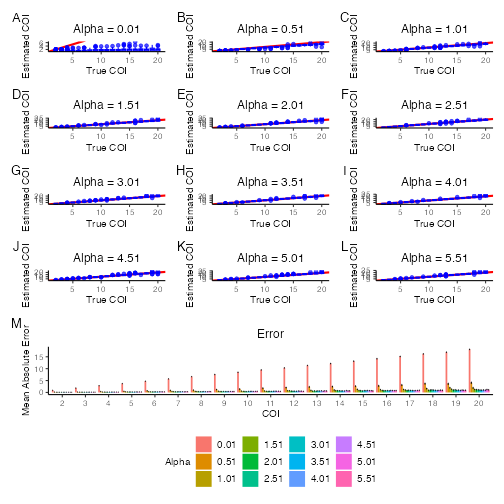
Overdispersion
tover <- cont_sensitivity(
  coi = 2:20,
  overdispersion = seq(0, 0.25, 0.05),
  repetitions = 100,
  seq_error = 0.01,
  plmaf = p,
  coi_method = c("variant", "frequency")
)

tover_image <- sensitivity_plot(
  data = tover,
  result_type = "cont",
  title = "Predicted COI",
  dims = c(4, 3),
  sub_title = paste0(
    rep(c("Var, ", "Freq, "), each = 6),
    "Dispersion = ",
    seq(0, 0.25, 0.05)
  )
)

tover_error <- error_plot(
  tover,
  fill = "overdispersion",
  legend_title = "Overdispersion",
  title = "Error",
  second_fill = "coi_method"
)

tover_fig <- tover_image / tover_error +
  plot_annotation(
    tag_levels = "A",
    theme = theme(plot.tag = element_text(size = 10))
  ) +
  plot_layout(heights = c(5, 1)) +
  theme(legend.position = "bottom")

tover_fig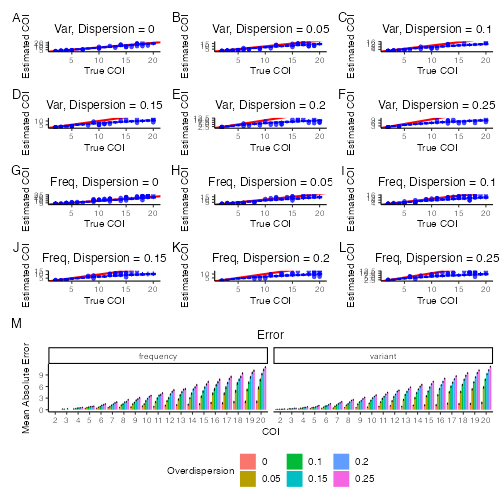
Relatedness
trelated <- cont_sensitivity(
  coi = 2:20,
  relatedness = seq(0, 0.5, 0.1),
  repetitions = 100,
  seq_error = 0.01,
  plmaf = p,
  coi_method = c("variant", "frequency")
)

trelated_image <- sensitivity_plot(
  data = trelated,
  result_type = "cont",
  title = "Predicted COI",
  dims = c(4, 3),
  sub_title = paste(
    paste0("Related =  ", seq(0, 0.5, 0.1)),
    rep(c("Variant Method", "Frequency Method"), each = 6),
    sep = ", "
  )
)

trelated_error <- error_plot(
  trelated,
  fill = "relatedness",
  legend_title = "Related",
  title = "Error",
  second_fill = "coi_method"
)

trelated_fig <- trelated_image / trelated_error +
  plot_annotation(
    tag_levels = "A",
    theme = theme(plot.tag = element_text(size = 10))
  ) +
  plot_layout(heights = c(6, 1)) +
  theme(legend.position = "bottom")

trelated_fig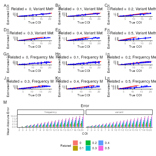
Epsilon
tepsilon <- cont_sensitivity(
  coi = 2:20,
  epsilon = seq(0, 0.025, 0.005),
  repetitions = 100,
  seq_error = 0.01,
  plmaf = p,
  coi_method = c("variant", "frequency")
)

tepsilon_image <- sensitivity_plot(
  data = tepsilon,
  result_type = "cont",
  title = "Predicted COI",
  dims = c(4, 3),
  sub_title = paste0(
    rep(c("Var, ", "Freq, "), each = 6),
    "Epsilon = ",
    seq(0, 0.025, 0.005)
  )
)

tepsilon_error <- error_plot(
  tepsilon,
  fill = "epsilon",
  legend_title = "Epsilon",
  title = "Error",
  second_fill = "coi_method"
)

tepsilon_fig <- tepsilon_image / tepsilon_error +
  plot_annotation(
    tag_levels = "A",
    theme = theme(plot.tag = element_text(size = 10))
  ) +
  plot_layout(heights = c(3, 1)) +
  theme(legend.position = "bottom")

tepsilon_fig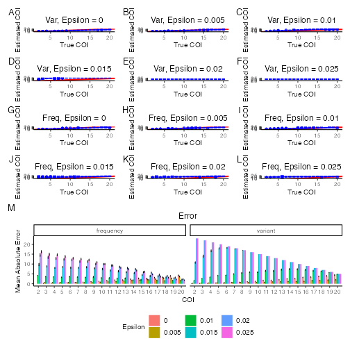
Estimation parameters
COI
tcoi <- cont_sensitivity(
  coi = 2:40,
  max_coi = 40,
  repetitions = 100,
  plmaf = p,
  seq_error = 0.01,
  coi_method = c("variant", "frequency")
)

tcoi_image <- sensitivity_plot(
  data = tcoi,
  dims = c(1, 2),
  result_type = "cont",
  title = "Predicted COI",
  sub_title = c("Variant Method", "Frequency Method")
)

tcoi_error <- error_plot(
  tcoi,
  fill = "coi_method",
  legend_title = "COI Method",
  title = "Error",
  fill_levels = c("Variant Method", "Frequency Method")
)

tcoi_fig <- tcoi_image / tcoi_error +
  plot_annotation(
    tag_levels = "A",
    theme = theme(plot.tag = element_text(size = 10))
  ) +
  theme(legend.position = "bottom")

tcoi_fig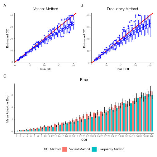
Sequencing error
tseq <- cont_sensitivity(
  coi = 2:20,
  epsilon = 0.01,
  seq_error = seq(0, 0.10, 0.02),
  repetitions = 100,
  plmaf = p,
  coi_method = c("variant", "frequency")
)

tseq_image <- sensitivity_plot(
  data = tseq,
  result_type = "cont",
  title = "Predicted COI",
  dims = c(4, 3),
  sub_title = paste0(
    rep(c("Variant, ", "Frequency, "), each = 6),
    "Seq Error = ",
    seq(0, 0.12, 0.02)
  )
)

tseq_error <- error_plot(
  tseq,
  fill = "seq_error",
  legend_title = "Sequence Error",
  title = "Error"
)

tseq_fig <- tseq_image / tseq_error +
  plot_annotation(
    tag_levels = "A",
    theme = theme(plot.tag = element_text(size = 10))
  ) +
  plot_layout(heights = c(5, 1)) +
  theme(legend.position = "bottom")

tseq_fig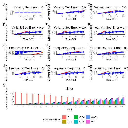
Bins
tbin <- cont_sensitivity(
  coi = 2:20,
  use_bins = c(TRUE, FALSE),
  plmaf = p,
  repetitions = 100,
  coi_method = c("variant", "frequency")
)

tbin_image <- sensitivity_plot(
  data = tbin,
  result_type = "cont",
  title = "Predicted COI",
  dims = c(2, 2),
  sub_title = paste(
    c("Variant Method,", "Frequency Method,"),
    "Bins =",
    rep(c(TRUE, FALSE), each = 2)
  )
)

tbin_error <- error_plot(
  tbin,
  fill = "use_bins",
  fill_levels = as.character(c(TRUE, FALSE)),
  legend_title = "COI Method",
  title = "Error",
  second_fill = "coi_method"
)

tbin_fig <- tbin_image / tbin_error +
  plot_annotation(
    tag_levels = "A",
    theme = theme(plot.tag = element_text(size = 10))
  ) +
  plot_layout(heights = c(3, 1)) +
  theme(legend.position = "bottom")

tbin_fig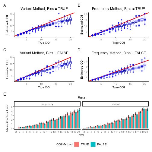
Bin size
tbin_size <- cont_sensitivity(
  coi = 2:20,
  use_bins = TRUE,
  bin_size = seq(10, 100, 30),
  plmaf = p,
  repetitions = 100,
  seq_error = 0.01,
  coi_method = c("variant", "frequency")
)

tbin_size_image <- sensitivity_plot(
  data = tbin_size,
  result_type = "cont",
  title = "Predicted COI",
  dims = c(2, 4),
  sub_title = rep(paste("Bin Size =", seq(10, 100, 30)), 2)
)

tbin_size_error <- error_plot(
  tbin_size,
  fill = "bin_size",
  fill_levels = as.character(seq(10, 100, 30)),
  legend_title = "COI Method",
  title = "Error"
)

tbin_size_fig <- tbin_size_image / tbin_size_error +
  plot_annotation(
    tag_levels = "A",
    theme = theme(plot.tag = element_text(size = 10))
  ) +
  plot_layout(heights = c(3, 1)) +
  theme(legend.position = "bottom")

tbin_size_fig